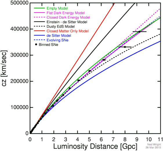
Several groups are measuring distant supernovae with the goal of determining whether the Universe is open or closed by measuring the curvature in the Hubble diagram. The figure below shows a binned version of the latest dataset: Betoule et al. (2014).
The curves show a closed Universe (Ω = 2) in red, the critical density Universe (Ω = 1) in black, the empty Universe (Ω = 0) in green, the steady state model in blue, and the WMAP based concordance model with ΩM = 0.27 and ΩV = 0.73 in purple. This model gives Ho = 71 km/sec/Mpc which has been used to scale the luminosity distances in the plot. The data show an accelerating Universe at low to moderate redshifts but a decelerating Universe at higher redshifts, consistent with a model having both a cosmological constant and a significant amount of dark matter. The dashed black curve shows an Einstein-de Sitter model with a constant co-moving dust density which can be ruled out. The dashed purple curve shows a closed ΛCDM model which is a good fit to the data. The dashed blue curve shows an evolving supernova model which is also a good fit. Note that power law a(t) models where the scale factor is a power of the cosmic time can be ruled out, although not by supernova data alone.
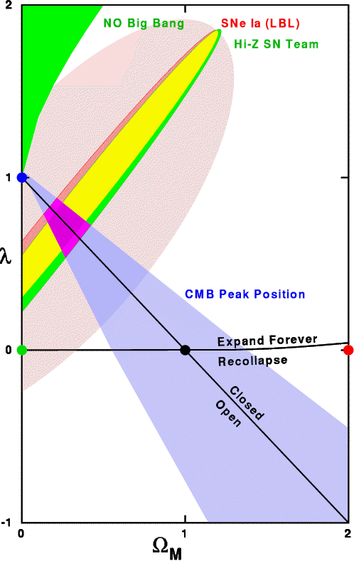 Both the Supernova Cosmology Project and the High-z Supernova Team
groups were the subject of news articles in Science, on 30 Jan
1998 and 27 Feb 1998. I have combined their two error ellipses along
with another constraint from the circa 1998
knowledge of the location of the acoustic peak in the
angular power spectrum of the CMB anisotropy. The two SNe groups gave
very similar error ellipses, and the combined CMB-SNe fit indicates that
a flat Universe with a
cosmological constant is preferred. But the
systematic errors on the SNe data, shown as the large grey (or pink) ellipse,
could allow for a vanishing cosmological constant lambda.
The red, black, green and blue circles on the Figure to the right are
keyed to the colors of the curves on the Figure shown above.
A larger GIF file or a
Postscript version of this figure are
available.
Both the Supernova Cosmology Project and the High-z Supernova Team
groups were the subject of news articles in Science, on 30 Jan
1998 and 27 Feb 1998. I have combined their two error ellipses along
with another constraint from the circa 1998
knowledge of the location of the acoustic peak in the
angular power spectrum of the CMB anisotropy. The two SNe groups gave
very similar error ellipses, and the combined CMB-SNe fit indicates that
a flat Universe with a
cosmological constant is preferred. But the
systematic errors on the SNe data, shown as the large grey (or pink) ellipse,
could allow for a vanishing cosmological constant lambda.
The red, black, green and blue circles on the Figure to the right are
keyed to the colors of the curves on the Figure shown above.
A larger GIF file or a
Postscript version of this figure are
available.
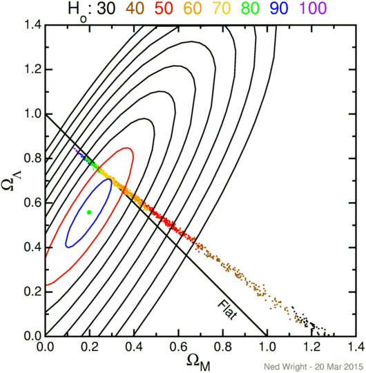 The supernova data in the JLA catalog published by Betoule
et al. (2014) provide the best fit, 1, 2 and 3..9 standard deviation
contours shown as the green dot and the blue, red and black ellipses in the
figure at left. The CMB data using WMAP 9 year results
provide the cloud of dots from a
Monte Carlo Markov chain sampling of the likelihood function.
The CMB degeneracy track does not follow the flat Universe line,
but crosses the flat line at a point reasonably consistent with the
supernova fit.
Each CMB model has an implied Hubble constant which provides the color code
for the dots. A model that fits both the supernova data and the CMB
data has a Hubble constant that agrees reasonably well
with the Hubble Space Telescope
Key Project value of the Hubble constant.
The supernova data in the JLA catalog published by Betoule
et al. (2014) provide the best fit, 1, 2 and 3..9 standard deviation
contours shown as the green dot and the blue, red and black ellipses in the
figure at left. The CMB data using WMAP 9 year results
provide the cloud of dots from a
Monte Carlo Markov chain sampling of the likelihood function.
The CMB degeneracy track does not follow the flat Universe line,
but crosses the flat line at a point reasonably consistent with the
supernova fit.
Each CMB model has an implied Hubble constant which provides the color code
for the dots. A model that fits both the supernova data and the CMB
data has a Hubble constant that agrees reasonably well
with the Hubble Space Telescope
Key Project value of the Hubble constant.
The addition of high redshift supernovae has had two effects on the supernova error ellipse. The long axis of the ellipse has gotten shorter, and the slope of the ellipse has gotten higher. The best fit model has gotten closer to the CMB degeneracy track in absolute terms, and it has also gotten closer in terms of standard deviations.
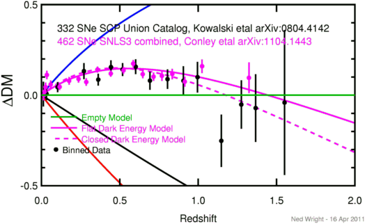
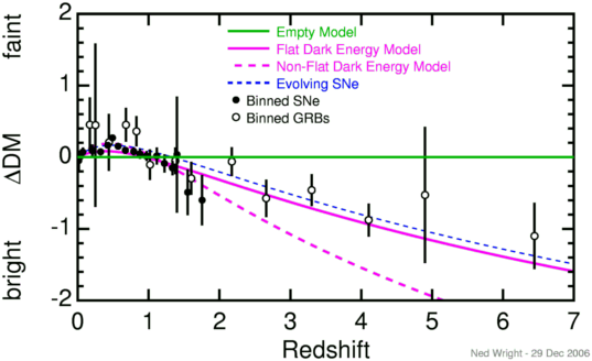
In the last few years distant supernovae with redshifts up to 1.755 have been
observed by the Hubble Space Telescope. These objects show that the trend
toward fainter supernovae seen at moderate redshifts has reversed. This
reversal means that one possible alternative to the accelerating
Universe as the explanation of the fainter supernovae at z near
0.5 can be rejected. This rejected alternative proposed that dust
between galaxies made the distant supernovae fainter by absorbing some
of their light, if the dust density scales like the matter density.
In the plot below, the brightness or faintness of
distant supernovae relative to the empty Universe model is plotted
vs redshift.
The Union 2.1 catalog, when binned to give normal points, gives this table:
  <z>  #    <ΔDM>     σ
0.0068 25  0.0057 0.0667
0.0117 25  0.0225 0.0422
0.0154 25 -0.0149 0.0338
0.0192 25 -0.0132 0.0291
0.0237 25 -0.0107 0.0255
0.0284 25  0.0439 0.0245
0.0331 25  0.0096 0.0229
0.0436 25 -0.0487 0.0209
0.0668 25 -0.0619 0.0189
0.1101 25  0.0198 0.0178
0.1581 25 -0.0084 0.0192
0.1991 25  0.0582 0.0194
0.2433 25  0.0532 0.0223
0.2790 25  0.0322 0.0224
0.3172 25  0.0411 0.0244
0.3564 25  0.0721 0.0242
0.3998 25  0.1400 0.0327
0.4383 25  0.0999 0.0284
0.4876 25  0.0492 0.0284
0.5435 25  0.0390 0.0275
0.5989 25  0.0750 0.0283
0.6671 25  0.0109 0.0323
0.7833 25  0.0845 0.0296
0.8912 25 -0.0487 0.0347
1.0386 22  0.0059 0.0372
1.2949 15  0.0248 0.0447
This data set is described in Suzuki et al. (2012).
The data points on the above plot come from my binning of the Conley et al. (2011) combined.dat file, which gives these normal points, where ΔDM is how much fainter the SNe are than expected in the empty or Milne model for the Universe:
  <z>      <ΔDM>     σ
0.01376   0.0001  0.0290
0.01970   0.0191  0.0256
0.02603   0.0450  0.0245
0.03432   0.1117  0.0230
0.05863   0.0588  0.0224
0.11585   0.0460  0.0183
0.17641   0.0794  0.0211
0.23664   0.0896  0.0205
0.28563   0.0729  0.0207
0.35740   0.1413  0.0166
0.44228   0.1194  0.0170
0.52328   0.1372  0.0184
0.58521   0.1740  0.0205
0.64596   0.1161  0.0230
0.71506   0.1019  0.0233
0.76831   0.1068  0.0275
0.83455   0.1168  0.0289
0.91428   0.0747  0.0278
1.02478   0.1598  0.0378
1.32375   0.0961  0.0845
and from my previous binning of the Kowalski et al. (2008) data set, which gives these normal points:
  <z>      <ΔDM>     σ
0.01165   0.0060  0.0678
0.03231   0.0074  0.0342
0.10263   0.0445  0.0281
0.27094   0.1330  0.0441
0.36235   0.0859  0.0326
0.44353   0.1551  0.0372
0.51734   0.1418  0.0356
0.60119   0.1570  0.0408
0.69209   0.0804  0.0499
0.80419   0.0885  0.0535
0.90584   0.0796  0.0804
0.99577   0.0995  0.0845
1.14750  -0.2520  0.1446
1.27500  -0.0517  0.1333
1.36667  -0.0710  0.1869
1.55100  -0.0407  0.4000
My binning of the Riess et al. (2007) data table gives these binned normal points:
   n   zmin    zmax     <z>      d(DM)   sigma
  31 0.00700 0.02100 0.01484  -0.0464  0.1383
  31 0.02300 0.05000 0.03352   0.0063  0.0691
  16 0.05100 0.12400 0.07131   0.0725  0.0644
   7 0.16000 0.24900 0.20671   0.0916  0.0878
  18 0.26300 0.35900 0.32239   0.0751  0.0506
  31 0.36900 0.46000 0.42323   0.1665  0.0406
  31 0.46100 0.52600 0.49016   0.2700  0.0395
  29 0.52600 0.62000 0.56921   0.1521  0.0375
  20 0.62700 0.72100 0.67190   0.0969  0.0478
  24 0.73000 0.83000 0.79029   0.0799  0.0519
  17 0.83200 0.93000 0.87647   0.0464  0.0697
  19 0.93500 1.02000 0.97011   0.0155  0.0696
   4 1.05600 1.14000 1.11400   0.0168  0.1179
   5 1.19000 1.26500 1.22280  -0.0870  0.1275
   6 1.30000 1.39000 1.33533  -0.1505  0.0998
   1 1.40000 1.40000 1.40000   0.0371  0.8100
   1 1.55100 1.55100 1.55100  -0.4897  0.3201
   1 1.75500 1.75500 1.75500  -0.5993  0.3501
where d(DM) is the difference between the distance modulus determined from the flux and the distance modulus computed from the redshift in the empty Universe model, and sigma is the standard deviation of the d(DM) in the bin. I use a robust statistical technique to get the binned values and therefore include both the Gold and Silver samples. I also include the low redshift supernovae which of course only affect the low z bin. But I have assumed a 1500 km/sec uncertainty in the redshift when computing the d(DM) which de-weights the low redshift bin.
I don't see much difference between the Gold+Silver data and the data restricted to Gold, but here is a binning of the Gold data alone:
   n   zmin    zmax     <z>      d(DM)   sigma
  22 0.01000 0.02100 0.01536   0.0186  0.1599
  22 0.02300 0.04000 0.02986   0.0441  0.0892
  18 0.04300 0.12400 0.06467   0.0387  0.0635
   4 0.17200 0.26300 0.21600   0.1356  0.0912
  12 0.27800 0.37100 0.33167   0.0720  0.0551
  22 0.38000 0.47000 0.43777   0.1798  0.0446
  22 0.47000 0.54000 0.50223   0.2119  0.0462
  22 0.54300 0.64000 0.59268   0.1092  0.0417
  11 0.64300 0.74000 0.69855   0.0930  0.0607
  18 0.75600 0.85400 0.81217   0.0422  0.0607
  13 0.86000 0.95400 0.91862   0.0140  0.0767
   8 0.96100 1.05600 0.99863   0.1141  0.0912
   4 1.12000 1.19900 1.14975  -0.0473  0.1273
   4 1.23000 1.30500 1.26625   0.0566  0.1138
   3 1.34000 1.39000 1.36667  -0.1848  0.1360
   1 1.75500 1.75500 1.75500  -0.5993  0.3501
I have also thrown the ESSENCE dataset into the Riess et al. (2007) dataset, getting the followed binned dataset. I needed to add 0.022 mag from the μ values in Table 9 of Wood-Vasey et al. (2007) to make the sample of objects in common consistent with the Riess et al. scale.
   n   zmin    zmax     <z>      d(DM)   sigma
  37 0.00700 0.02400 0.01589  -0.0518  0.1180
  37 0.02450 0.05800 0.03757   0.0040  0.0573
  12 0.06100 0.16000 0.09475   0.1026  0.0752
  14 0.17200 0.26800 0.22071   0.1097  0.0625
  36 0.27400 0.37100 0.32989   0.0963  0.0374
  37 0.37400 0.45500 0.42224   0.1698  0.0373
  37 0.45900 0.51100 0.48408   0.2449  0.0371
  37 0.51400 0.61000 0.55297   0.1687  0.0340
  31 0.61200 0.71000 0.65503   0.0999  0.0358
  21 0.71900 0.81800 0.77471   0.0535  0.0526
  20 0.82200 0.91000 0.85905   0.0546  0.0644
  21 0.92700 1.02000 0.96614   0.0469  0.0677
   4 1.05600 1.14000 1.11400   0.0168  0.1179
   5 1.19000 1.26500 1.22280  -0.0870  0.1275
   6 1.30000 1.39000 1.33533  -0.1505  0.0998
   1 1.40000 1.40000 1.40000   0.0371  0.8100
   1 1.55100 1.55100 1.55100  -0.4897  0.3201
   1 1.75500 1.75500 1.75500  -0.5993  0.3501
The table above is Table 1 from Wright (2007).
The table below is the Riess et al Gold plus the ESSENCE supernovae, from Table 2 in Wright (2007):
   n   zmin    zmax     <z>      d(DM)   sigma
  29 0.01000 0.02500 0.01694  -0.0351  0.1250
  29 0.02500 0.05300 0.03612   0.0240  0.0667
  10 0.05600 0.12400 0.07760   0.0742  0.0798
  10 0.15900 0.24900 0.20320   0.1229  0.0735
  27 0.26300 0.36300 0.31963   0.1054  0.0425
  29 0.36800 0.45000 0.41490   0.1437  0.0390
  29 0.45500 0.50800 0.48083   0.2032  0.0401
  29 0.51000 0.60400 0.55145   0.1386  0.0389
  25 0.61000 0.70700 0.64748   0.1190  0.0381
  18 0.73000 0.83000 0.78883   0.0581  0.0587
  10 0.83200 0.90500 0.86660   0.0073  0.0811
  14 0.93500 1.02000 0.96957   0.0347  0.0760
   4 1.05600 1.14000 1.11400   0.0168  0.1179
   3 1.19900 1.23000 1.21967   0.0806  0.1434
   5 1.30000 1.39000 1.34100  -0.1629  0.1054
   1 1.75500 1.75500 1.75500  -0.5993  0.3501
Note that this Riess etal (2007) dataset is a compilation of data from many sources and there are indications that there are systematic differences between these subsets.
Observationally
d(DM) = 5 log (Ho sqrt[L/(4πF)]/[cz(1+z/2)])while theoretically
d(DM) = 5 log[Z(z) J([1-Ωtot]Z(z)2) (1+z)/(z(1+z/2))]with Z(z) and J(x) defined here. The Hubble constant used in computing the empty Universe Milne model which is subtracted off is 63.8 km/sec/Mpc, to be consistent with Riess et al. (2007). Note that any fit to this dataset should include as a free parameter an adjustment to this Hubble constant, which gives a constant term in d(DM).
I found the following chi2 values for fits to both the unbinned and the binned Riess et al. (2007) Gold+Silver data:
                                                unbinned        binned
Name            Omega_m         Omega_vac       chi^2/df        chi^2/df
Best fit        0.55            1.15            290.4/289       12.1/15
Best flat       0.36            0.64            297.7/290       20.1/16
WMAP model      0.27            0.73            302.6/291       25.3/17
Milne           0.0             0.0             321.2/291       44.5/17
EdS             1.0             0.0             386.3/291      108.6/17
Evolving        1.0             0.0             295.8/290       18.2/16
I have also binned the γ-ray burst (GRB) data from Schaefer (2006):
   n   zmin    zmax     <z>      d(DM)   sigma
   1 0.17000 0.17000 0.17000   0.4532  0.3813
   1 0.25000 0.25000 0.25000   0.4471  1.1402
   2 0.43000 0.45000 0.44000   0.2069  0.3973
   6 0.61000 0.71000 0.68000   0.4517  0.2367
   7 0.78000 0.86000 0.82857   0.3608  0.2116
   6 0.96000 1.10000 1.02000  -0.1046  0.2142
   8 1.24000 1.51000 1.37625  -0.0509  0.1866
   5 1.52000 1.71000 1.60200  -0.2954  0.2299
   8 1.98000 2.35000 2.17375  -0.0616  0.2020
   7 2.44000 2.90000 2.65857  -0.5738  0.2612
   8 3.08000 3.53000 3.30000  -0.4595  0.2219
   7 3.79000 4.50000 4.10429  -0.8771  0.2301
   1 4.90000 4.90000 4.90000  -0.5275  0.9500
   2 6.29000 6.60000 6.44500  -1.1004  0.4628
Note that Schaefer uses a different Ho than Riess but I have used the appropriate Ho (72 km/sec/Mpc) when computing the Milne model for this dataset.
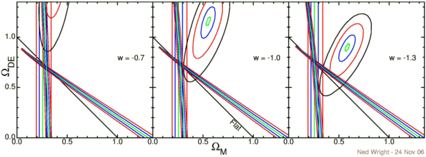
With multiple datasets it is now possible to say something about
the equation of state parameter w
even without assuming the Universe is flat. The figure below shows
the constraints from the Hubble constant (vertical lines), the
baryon acoustic oscillations
(nearly vertical lines),
the CMB (tilted fan of lines), and the supernovae (ellipses).
In each case green is right on (or 0.3 sigma for the supernovae),
blue is 1 sigma, red is 2 sigma, and black is 3 sigma.
Ho taken to be 71 +/- 5 km/sec/Mpc
based on an average of the
HST Key project, the
SZ effect, the
Cepheids
in the nuclear maser ring galaxy NGC 4258, and the
double-lined eclipsing binary
in M33.
FAQ | Tutorial : Part 1 | Part 2 | Part 3 | Part 4 | Age | Distances | Bibliography | Relativity
© 1997-2015 Edward L. Wright. Last modified 01 Apr 2015