It is almost impossible to tell the distances of objects we see in the sky. Almost, but not quite, and astronomers have developed a large variety of techniques. Here I will describe 26 of them. I will ignore the work that went into determining the astronomical unit: the scale factor for the Solar System, and just consider distances outside of the Solar System.
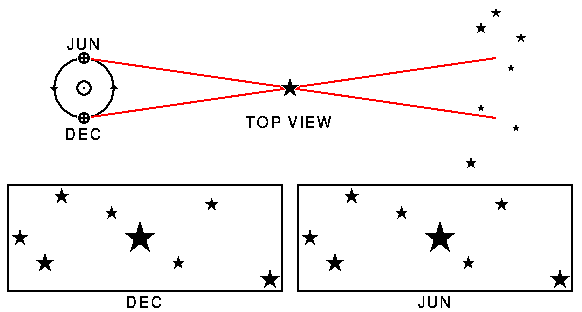
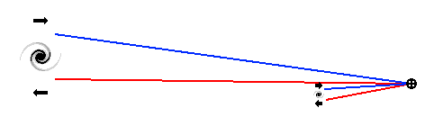
This method rates an A because it is the gold standard for astronomical
distances. It is based on measuring two angles and the included side
of a triangle formed by 1) the star, 2) the Earth on one side of its
orbit, and 3) the Earth six months later on the other side of its orbit.
The parallax of a star is one-half the angle at the star in the diagram above. Thus the parallax is the angle at the star in an Earth-Sun-star triangle. Since this angle is always very small, the sine and tangent of the parallax are very well approximated by the parallax angle measured in radians. Therefore the distance to a star is
D[in cm] = [Earth-Sun distance in cm]/[parallax in radians]Astronomers usually say the Earth-Sun distance is 1 astronomical unit, where 1 au = 1.5E13 cm, and measure small angles in arc-seconds. [Note that 1.5E13 is computerese for 15,000,000,000,000] One radian has 648000/pi arc-seconds. If we use these units, the unit of distance is [648000/pi] au = 3.085678E18 cm = 1 parsec. A star with a parallax of 1 arc-second has a distance of 1 parsec. No known stars have parallaxes this big. Proxima Centauri has a parallax of 0.76". [The double quote is used to denote arc-seconds (as well as inches).]
The first stellar parallax (of the star 61 Cygni) was measured by Friedrich Wilhelm Bessel (1784-1846) in 1838. Bessel is also known for the Bessel functions in mathematical physics.
Not many stars are close enough to have useful trigonometric parallaxes.
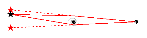
But when stars are in a stable star cluster whose physical size is not
changing, like the
Pleiades,
then the apparent motions of the stars within the cluster
can be used to determine the distance to the cluster.
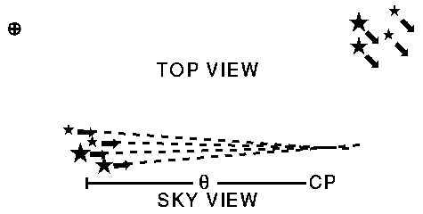
D[in cm] = VT[in cm/sec]/[d(theta)/dt]

D[in pc] = (VR/4.74 km/sec)*tan(theta)/{d(theta)/dt[in "/yr]}
The odd constant 4.74 km/sec is one au/year.
Because a time interval of 100 years can be used to measure d(theta)/dt,
precise distances to nearby star clusters are possible.
This method has been applied to the
Hyades cluster giving a distance of 45.53 +/- 2.64 pc.
The average of HIPPARCOS
trigonometric parallaxes for Hyades members gives a
distance of 46.34 +/- 0.27 pc
(Perryman et
al.).
Another method can be used to measure the average distance to a set of
stars, chosen to be all about the same distance from the Earth.
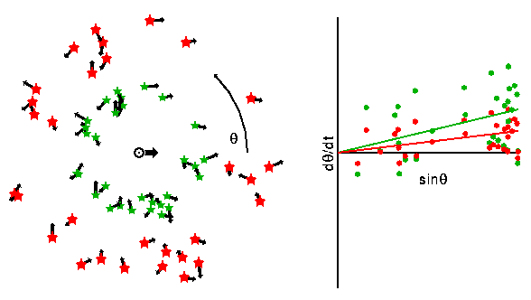
D[in cm] = V(sun)[in cm/sec]/(mu [in radians/sec])

D[in pc] = 4.16/(mu [in "/yr])
where the odd constant 4.16 is the Solar motion in au/yr.
When the stars have measured radial velocities, then the scatter in their proper motions can be used to determine the mean distance. It is
                  (scatter in VR)[in cm/sec]
D[in cm] = ----------------------------------------
           (scatter in d(theta)/dt)[in radians/sec]
The pattern of differential rotation in our galaxy can be used to determine the distance of a source when its radial velocity is known.
The distance to an expanding object like a supernova remnant such as Tycho can be determined by measuring:
The distance is then calculated using
D = VR/d(theta)/dt with theta in radiansThis method is subject to a systematic error when the velocity of the material behind the shock is less than the velocity of the shock. In supernova remnants in the adiabatic phase this is in fact the case, with VR = 0.75 V(shock), so the calculated distance can be too small by 25%.
The center elliptical ring around SN1987A in the LMC appears to be due to an inclined circular ring around the progenitor. When the pulse of ultraviolet light from the supernova hit the ring, it lit up in ultraviolet emission lines which were observed by the International Ultraviolet Explorer (IUE). The first detection of these lines at time, t1, and also the time when the lines from the last part of the ring to be illuminated, t2, were both clearly evident in the IUE light curve of the UV lines. If t0 is the time that we first saw the supernova, then the extra light travel times to the front and back of the ring are:
t1 - t0 = R(1 - sin(i))/c
t2 - t0 = R(1 + sin(i))/c
where R is the radius of the ring in cm. Thus
R = c(t1-t0 + t2-t0)/2When the HST was launched it took a picture of SN 1987A and saw the ring, and measured the angular radius of the ring, theta. The ratio gives the distance:
D = R/theta with theta in radiansApplied to the LMC using SN 1987A one gets D = 47 +/- 1 kpc, based on t1-t0 = 75 +/- 2.6 days, t2 - t0 = 390 +/- 1.8 days, and a ring angular semimajor axis of 0.858 arc-seconds. (Gould 1995, ApJ, 452, 189) This method is basically the expansion method applied to the expansion of the shell of supernova radiation that expands at the speed of light. It can be applied to other known geometries, as well.
If a binary orbit is observed both visually and spectroscopically, then both the angular size and the physical size of the orbit are known. The ratio gives the distance.

The Baade-Wesselink method is applied to pulsating stars. Using the color and flux light curves, one finds the ratio of the radii at different times:
              sqrt[Flux(t2)/SB(Color(t2)]
R(t2)/R(t1) = ---------------------------
              sqrt[Flux(t1)/SB(Color(t1)]
Then spectra of the star throughout its pulsation period are used
to find its radial velocity Vr(t). Knowing how fast the
star's surface is moving, one finds
R(t2)-R(t1) by adding up velocity*time during the time interval
between t1 and t2. If you know both the ratio of the radii
R(t2)/R(t1) from fluxes and colors and the difference in the
radii R(t2)-R(t1) from spectroscopy, then you have two
equations in two unknowns and it is easy to solve for the radii.
With the radius and angle, the distance is found
using D = R/theta.
In a double-lined spectroscopic binary, the projected size of the orbit a*sin(i) is found from the radial velocity amplitude and the period. In an eclipsing binary, the relative radii of the stars R1/a and R2/a and the inclination of the orbit i are found by analyzing the shapes of the eclipse light curves. Using the observed fluxes and colors to get surface brightnesses, the angular radii of the stars can be estimated. R1 is found from i, a*sin(i) and R1/a; and with theta1 the distance can be found.
For the hot O stars in the binary used to measure the distance to M33 the atmosphere contains a large number of free electrons. These scatter and reflect light without changing the spectrum. Thus the surface brightness can be lower than the surface brightness expected from the colors and line ratios if there is a larger than expected amount of electron scattering. The calculated distance would then be too large.
The Baade-Wesselink method can be applied to an expanding star: the variations in radius do not have to be periodic. It has been applied to Type II supernovae, which are massive stars with a hydrogen rich envelope that explode when their cores collapse to form neutron stars. It can also be applied to Type Ia supernovae, but these objects have no hydrogen lines in their spectra. Since the surface brightness vs color law is calibrated using normal, hydrogen-rich stars, the EPM is normally used on hydrogen-rich supernovae, which are Type II. The Type II SN1987A in the Large Magellanic Cloud has been used to calibrate this distance indicator.
D = sqrt[L/(4*pi*F)]
When distances to nearby stars were found using trigonometric parallaxes in the late 19th and early 20th century, it became possible to study the luminosities of stars. Einar Hertzsprung and Henry Norris Russell both plotted stars on a chart of luminosity and temperature. Most stars fall on a single track, known as the Main Sequence, in this diagram, which is now known as the H-R diagram after Hertzsprung and Russell. Often the absolute magnitude is used instead of the luminosity, and the spectral type or color is used instead of the temperature.
When looking at a cluster of stars, the apparent magnitudes and colors of the stars form a track that is parallel to the Main Sequence, and by correctly choosing the distance, the apparent magnitudes convert to absolute magnitudes that fall on the standard Main Sequence.
When the spectrum of a star is observed carefully, it is possible to determine two parameters of the star as well as the chemical abundances in the star's atmosphere. The first of these two parameters is the surface temperature of the star, which determines the spectral type in the range OBAFGKM from hottest to coolest. The hot O stars show ionized helium lines, the B stars show neutral helium lines, the A stars have strong hydrogen lines, the F and G stars have various metal lines, and the coolest K and M stars have molecular bands. The spectral classes are further subdivided with a digit, so the Sun is a G2 star.
The second parameter that can be determined is the surface gravity of
the star. The higher the surface gravity, the higher the pressure in
the atmosphere, and high pressure leads to line broadening and also
reduces the amount of ionization in the atmosphere.
The surface gravity is denoted by the
L = 4*pi*sigma*T4*R2
L = A*Mb                      Mass-luminosity law with b = 3-4
g = G*M/R2
Given the temperature from the spectral type, and the surface gravity
from the luminosity class, these equations can be used to find the
mass and luminosity. If the luminosity and flux are known the distance
follows from the inverse square law.
One warning about this method: it only works for normal stars, and any given single object might not be normal. Main sequence fitting in a cluster is much more reliable since with a large number of stars it is easy to find the normal ones.
Cepheid
variable stars
are pulsating stars, named after the first known
member of the class, Delta Cephei. These stars pulsate because the
hydrogen and helium ionization zones are close to the surface of the
star. This more or less fixes the temperature of the variable star,
and produces an instability strip in the H-R diagram.
L = Const * V(rot)4Since the rotational velocity of a spiral galaxy can be measured using an optical spectrograph or radio telescopes, the luminosity can be determined. Combined with the measured flux, this luminosity gives the distance. The diagram below shows two galaxies: a giant spiral and a dwarf spiral, but the small galaxy is closer to the Earth so they both cover the same angle on the sky and have the same apparent brightness.
L = Const * sigma(v)4Since the velocity dispersion of an elliptical galaxy can be measured using an optical spectrograph, the luminosity can be determined. Combined with the measured flux, this luminosity gives the distance.
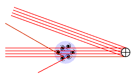
When a quasar is viewed through a
gravitational
lens, multiple images are seen, as shown in diagram below.
Hot gas in clusters of galaxies distorts the spectrum of the cosmic
microwave background observed through the cluster.
The diagram below shows a sketch of this process. The hot electrons
in the cluster of galaxies scatter a small fraction of the cosmic
microwave background photons and replace them with slightly higher
energy photons.
The X-ray emission, IX, from the hot gas in the cluster is proportional to (1) the square of the number density of electrons, (2) the thickness of the cluster along our line of sight, and (3) depends on the electron temperature and X-ray frequency. As a result, the ratio
y2/IX = CONST * (Thickness along LOS) * f(T)If we assume that the thickness along the LOS is the same as the diameter of the cluster, we can use the observed angular diameter to find the distance.
This technique is very difficult, and years of hard work by pioneers like Mark Birkinshaw yielded only a few distances, and values of Ho that tended to be on the low side. Recent work with close packed radio interferometers operating at 30 GHz has given precise measurements of the radio brightness decrement for 18 clusters, but only a few of these have adequate X-ray data. A recent Sunyaev-Zeldovich determination of the Hubble constant gave 77 +/- 10 km/sec/Mpc from 38 clusters.
Big new instruments for measuring the Sunyaev-Zeldovich effect include the South Pole Telescope the SZA, and the Atacama Cosmology Telescope.
The Doppler shift gives the redshift of a distant object which is our best indicator of its distance, but we need to know the Hubble constant, Ho. Then
D = VR/HoBut the measured value of the Hubble constant has changed by a factor of 8 since Hubble's work, as discussed in Huchra's Ho history.
But wait, there's MORE! Pulsar dispersion measures and interstellar extinction increase with distance along a given line of sight and can be used to determine distances. The peak luminosity of a classical nova can be estimated from its rate of decay, but the variation has the opposite sense to that of Type Ia SNe: more luminous novae decay more rapidly. The globular cluster luminosity function can be used to estimate the distance to a galaxy from the observed brightness of its globular clusters.
Tutorial:
Part 1 |
Part 2 |
Part 3 |
Part 4
FAQ |
Age |
Distances |
Bibliography |
Relativity
© 1997-2018 Edward L. Wright. Last modified 07 Sep 2018