Cosmology Tutorial

Previous Section

Part 1: Observations of Global Properties
Part 2: Homogeneity and Isotropy; Many Distances; Scale Factor
Part 3: Spatial Curvature; Flatness-Oldness; Horizon
Part 4: Inflation; Anisotropy and Inhomogeneity

Inflation

The "inflationary scenario", developed by Starobinsky and by Guth, offers a solution to the flatness-oldness problem and the horizon problem. The inflationary scenario invokes a vacuum energy density. We normally think of the vacuum as empty and massless, and we can determine that the density of the vacuum is less than 10^-29 gm/cc now. But in quantum field theory, the vacuum is not empty, but rather filled with virtual particles:

The space-time diagram above shows virtual particle-antiparticle pairs forming out of nothing and then annihilating back into nothing. For particles of mass m, one expects about one virtual particle in each cubical volume with sides given by the Compton wavelength of the particle, h/mc, where h is Planck's constant. Thus the expected density of the vacuum is rho = m⁴*c³/h³ which is rather large. For the largest elementary particle mass usually considered, the Planck mass M defined by 2*pi*G*M² = h*c, this density is 2*10⁹¹ gm/cc. That's a 2 followed by 91 zeroes! Thus the vacuum energy density is at least 120 orders of magnitude smaller than the naive quantum estimate, so there must be a very effective suppression mechanism at work. If a small residual vacuum energy density exists now, it leads to a "cosmological constant" which is one proposed mechanism to relieve the tight squeeze between the Omega_o=1 model age of the Universe, t_o = (2/3)/H_o = 9 Gyr, and the apparent age of the oldest globular clusters, 12-14 Gyr. The vacuum energy density can do this because it produces a "repulsive gravity" that causes the expansion of the Universe to accelerate instead of decelerate, and this increases t_o for a given H_o.

The inflationary scenario proposes that the vacuum energy was very large during a brief period early in the history of the Universe. When the Universe is dominated by a vacuum energy density the scale factor grows exponentially, a(t) = exp(H(t-t_o)). The Hubble constant really is constant during this epoch so it doesn't need the "naught". If the inflationary epoch lasts long enough the exponential function gets very large. This makes a(t) very large, and thus makes the radius of curvature of the Universe very large. The diagram below shows our horizon superimposed on a very large radius sphere on top, or a smaller sphere on the bottom. Since we can only see as far as our horizon, for the inflationary case on top the large radius sphere looks almost flat to us.

This solves the flatness-oldness problem as long as the exponential growth during the inflationary epoch continues for at least 100 doublings. Inflation also solves the horizon problem, because the future lightcone of an event that happens before inflation is expanded to a huge region by the growth during inflation.
Inflationary space-time diagram

This space-time diagram shows the inflationary epoch tinted green, and the future lightcones of two events in red. The early event has a future lightcone that covers a huge area, that can easily encompass all of our horizon. Thus we can explain why the temperature of the microwave background is so uniform across the sky.

Details: Large-Scale Structure and Anisotropy

Of course the Universe is not really homogeneous, since it contains dense regions like galaxies and people. These dense regions should affect the temperature of the microwave background. Sachs and Wolfe (1967, ApJ, 147, 73) derived the effect of the gravitational potential perturbations on the CMB. The gravitational potential, phi = -GM/r, will be negative in dense lumps, and positive in less dense regions. Photons lose energy when they climb out of the gravitational potential wells of the lumps:

Sachs-Wolfe effect conformal space-time diagram

This conformal space-time diagram above shows lumps as gray vertical bars, the epoch before recombination as the hatched region, and the gravitational potential as the color-coded curve phi(x). Where our past lightcone intersects the surface of recombination, we see a temperature perturbed by dT/T = phi/(3*c²). Sachs and Wolfe predicted temperature fluctuations dT/T as large as 1 percent, but we know now that the Universe is far more homogeneous than Sachs and Wolfe thought. So observers worked for years to get enough sensitivity to see the temperature differences around the sky. The first anisotropy to be detected was the dipole anisotropy by Conklin in 1969:

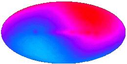
The map above is from COBE and is much better than Conklin's 2 standard deviation detection. The red part of the sky is hotter by (v/c)*T_o, while the blue part of the sky is colder by (v/c)*T_o, where the inferred velocity is v = 368 km/sec. This is how we measure the velocity of the Solar System relative to the observable Universe. It was another 23 years before the anisotropy predicted by Sachs and Wolfe was detected by Smoot et al. (1992, ApJL, 396, 1). The amplitude was 1 part in 100,000 instead of 1 part in 100, but was perfectly consistent with Lambda-CDM [Wright et al. 1992, ApJL, 396, 13].

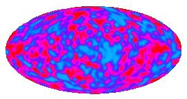
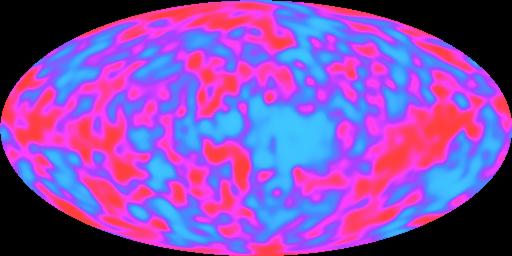
The map above shows cosmic anisotropy (and detector noise) after the dipole pattern and the radiation from the Milky Way have been subtracted out. The anisotropy in this map has an RMS value of 30 microK, and if it is converted into a gravitational potential using Sachs and Wolfe's result and that potential is then expressed as a height assuming a constant acceleration of gravity equal to the gravity on the Earth, we get a height of twice the distance from the Earth to the Sun. The "mountains and valleys" of the Universe are really quite large.

Inflation predicts a certain statistical pattern in the anisotropy. The quantum fluctuations normally affect very small regions of space, but the huge exponential expansion during the inflationary epoch makes these tiny regions observable.

Inflation generating equal power on all scales

The space-time diagram on the left above shows the future lightcones of quantum fluctuation events. The top of this diagram is really a volume which intersects our past lightcone making the sky. The future lightcones of events become circles on the sky. Events early in the inflationary epoch make large circles on the sky, as shown in the bottom map on the right. Later events make smaller circles as shown in the middle map, but there are more of them so the sky coverage is the same as before. Even later events make many small circles which again give the same sky coverage as seen on the top map.

An animated GIF file showing the spatial part of the above space-time diagram as a function of time is available here [1.2 MB].

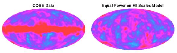
The pattern formed by adding all of the effects from events of all ages is known as "equal power on all scales", and it agrees with the COBE data.

Having found that the observed pattern of anisotropy is consistent with inflation, we can also ask whether the amplitude implies gravitational forces large enough to produce the observed clustering of galaxies.

phi(x) to clustering conformal space-time diagram

The conformal space-time diagram above shows the phi(x) at recombination determined by COBE's dT data, and the worldlines of galaxies which are perturbed by the gravitational forces produced by the gradient of the potential. Matter flows "downhill" away from peaks of the potential (red spots on the COBE map), producing voids in the current distribution of galaxies, while valleys in the potential (blue spots) are where the clusters of galaxies form.

COBE was not able to see spots as small as clusters or even superclusters of galaxies, but if we use "equal power on all scales" to extrapolate the COBE data to smaller scales, we find that the gravitational forces are large enough to produce the observed clustering, but only if these forces are not opposed by other forces. If the all the matter in the Universe is made out of the ordinary chemical elements, then there was a very effective opposing force before recombination, because the free electrons which are now bound into atoms were very effective at scattering the photons of the cosmic background. We can therefore conclude that most of the matter in the Universe is "dark matter" that does not emit, absorb or scatter light. Furthermore, observations of distant supernovae have shown that most of the energy density of the Universe is a vacuum energy density (a "dark energy") like Einstein's cosmological constant that causes an accelerating expansion of the Universe. These strange conclusions have been greatly strengthened by temperature anisotropy data at smaller angular scales which was provided by the Wilkinson Microwave Anisotropy Probe (WMAP) in 2003.

Ned Wright's home page