The BOOMERanG balloon-borne CMB anisotropy experiment observed 3% of the sky during a long duration flight in Antarctica. This region is shown in the all sky equal area Mollweide projection above. Here is a .tar.gz file containing data files extracted from Figure 1 of the first BOOMERanG paper. Save this file to disk, run it through gunzip and extract the files from the tar archive giving
126058 Jan  1 10:54 BOOMERanG_150.rle
126723 Jan  1 10:54 BOOMERanG_240.rle
125020 Jan  1 09:50 BOOMERanG_90.rle
 31719 Jan 25 23:34 DASI.rle
These files can be read using the following FORTRAN fragment:
      PARAMETER (IRES=8, NPIX= 12*4**IRES)
      REAL*4 SKY(NPIX)
      INTEGER LIST(19)
C
      OPEN (UNIT=1,FILE='BOOMERanG_90.rle',STATUS='OLD')
10    READ (1,900,END=20) NC,LIST
900   FORMAT(Q,I6,18I4)
      N = NC/4
      DO I=2,N
        SKY(LIST(1)+I-1) = 0.001*(LIST(I)-500)
      ENDDO
      GO TO 10
20    CLOSE (UNIT=1)
C
And the resulting array SKY contains the temperature in mK in each
of the 786432 HEALpix res 8 pixels. The value for pixel number I
is in SKY(I+1). The pixels are defined in galactic coordinates.
Pixels not observed by BOOMERanG or
obscured by the grid lines in the figure are left unchanged, so be sure
to allow for unobserved parts of the sky.
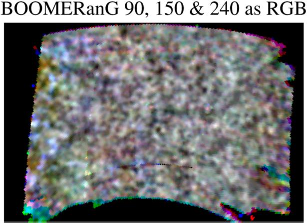
The paper states that these maps were smoothed to 22.5' =
0.375o. The pixel size in the JPEG file is
0.18o. I have further smoothed the maps with a 1.5 pixel
boxcar while repixelizing in HEALpix. Finally an unspecified amount
of large scale structure was filtered out of the BOOMERanG data
when Figure 1 was made. The image below shows an RGB
picture constructed from these files. I can clearly see the remains of
the grid lines and other flaws, so please use these files for
entertainment purposes only.
The file DASI.rle of course contains the DASI data from Figure 6 of
Leitch et
al. This is plotted in an (l,b) Mollweide projection below:
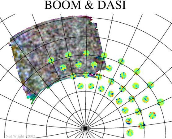
 An example of the kind of entertainment that can be had using these
files is the plot at right. It shows the cross-correlation of
BOOMERanG at 90 GHz and DASI at 30 GHz compared
to the autocorrelations of the two experiments in the 8 DASI spots that
substantially overlap the BOOMERanG field.
A constant plus a 2D gradient was fit to the data in each DASI spot
for both the DASI and the BOOMERanG data before the cross-correlation
and auto-correlations were computed.
There is a very substantial correlation between the two maps, so BOOMERanG
and DASI were both measuring real signals and the maps are correctly
aligned. The BOOMERanG autocorrelation shows an additional signal that
is not correlated with DASI which is probably noise and stripes in the
BOOMERanG map.
An example of the kind of entertainment that can be had using these
files is the plot at right. It shows the cross-correlation of
BOOMERanG at 90 GHz and DASI at 30 GHz compared
to the autocorrelations of the two experiments in the 8 DASI spots that
substantially overlap the BOOMERanG field.
A constant plus a 2D gradient was fit to the data in each DASI spot
for both the DASI and the BOOMERanG data before the cross-correlation
and auto-correlations were computed.
There is a very substantial correlation between the two maps, so BOOMERanG
and DASI were both measuring real signals and the maps are correctly
aligned. The BOOMERanG autocorrelation shows an additional signal that
is not correlated with DASI which is probably noise and stripes in the
BOOMERanG map.
Tutorial:
Part 1 |
Part 2 |
Part 3 |
Part 4
FAQ |
Age |
Distances |
Bibliography |
Relativity
© 2002 Edward L. Wright. Last modified 5 Feb 2002