Previous Section
Part 1: Observations of Global Properties
Part 2: Homogeneity and Isotropy; Many Distances; Scale Factor
Part 3: Spatial Curvature; Flatness-Oldness; Horizon
Part 4: Inflation; Anisotropy and Inhomogeneity
FAQ |
Tutorial :
Part 1 |
Part 2 |
Part 3 |
Part 4 |
Age |
Distances |
Bibliography |
Relativity
Spatial Curvature
One consequence of general relativity is that the curvature of space
depends on the ratio of
rho to
rho(crit). We call this ratio
Ω = rho/rho(crit). For Ω less than 1, the Universe has
negatively curved or
hyperbolic geometry. For Ω = 1, the Universe has Euclidean
or flat geometry. For Ω greater than 1, the Universe has
positively curved or spherical geometry. We have already seen
that the zero density case has hyperbolic geometry, since the cosmic
time slices in the special relativistic coordinates were hyperboloids
in this model.
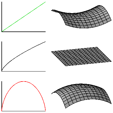
The figure above shows the three curvature cases plotted along side of
the corresponding a(t)'s. These a(t) curves assume that the
cosmological constant is zero, which
is not the current standard model. Ω > 1 still corresponds to
a spherical shape, but could expand forever even though the density is
greater than the critical density because of the repulsive gravitational
effect of the cosmological constant.
The age of the Universe
depends on Ωo as well as Ho. For Ω=1,
the critical density case, the scale factor is
a(t) = (t/to)2/3
and the age of the Universe is
to = (2/3)/Ho
while in the zero density case, Ω=0, and
a(t) = t/to with to = 1/Ho
If Ωo is greater than 1 the age of the Universe is even smaller
than (2/3)/Ho.
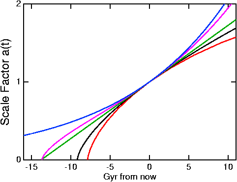
The figure above shows the scale factor vs time measured from the
present for Ho = 71 km/sec/Mpc and for
Ωo = 0 (green),
Ωo = 1 (black),
and Ωo = 2 (red) with no vacuum energy;
the WMAP model with ΩM= 0.27 and ΩV = 0.73
(magenta); and the Steady State model with ΩV = 1 (blue).
The ages of the Universe in these five models
are 13.8, 9.2, 7.9, 13.7 and infinity Gyr.
The recollapse of the Ωo = 2
model occurs when the Universe is 11 times older than it is
now, and all observations indicate Ωo < 2, so we have at least
80 billion more years before any Big Crunch.
The value of Ho*to
is a dimensionless number that should be 1 if
the Universe is almost empty and 2/3 if the Universe has the critical
density. In 1994 Freedman et al. (Nature, 371, 757) found
Ho = 80 +/- 17 and
when combined with
to = 14.6 +/- 1.7 Gyr, we find that
Ho*to = 1.19 +/- 0.29.
At face value this favored the empty Universe
case, but a 2 standard deviation error in the downward direction would
take us to the critical density case. Since both the age of globular
clusters used above and the value of Ho
depend on the distance scale in
the same way, an underlying error in the distance scale could make a
large change
in Ho*to.
In fact, recent data from the
HIPPARCOS
satellite
suggest that the Cepheid distance scale must be increased by 10%,
and also that the
age of globular clusters
must be reduced by 20%. If we take the latest
HST value for Ho = 72 +/- 8 (Freedman et al. 2001,
ApJ, 553, 47) and the latest globular cluster ages giving
to = 13.5 +/- 0.7 Gyr, we find that
Ho*to = 0.99 +/- 0.12 which is
consistent with an empty Universe, but also consistent with the
accelerating Universe that is the current standard model.
Flatness-Oldness Problem
However, if Ωo is sufficiently greater than 1,
the Universe will eventually
stop expanding, and then Ω will become infinite. If Ωo is
less than 1, the Universe will expand forever and the density goes
down faster than the critical density so Ω gets smaller and smaller.
Thus Ω = 1 is an unstable stationary point unless the expansion of the
universe is accelerating, and it is quite
remarkable that Ω is anywhere close to 1 now.
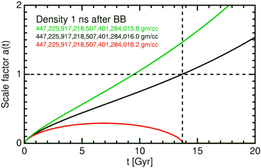
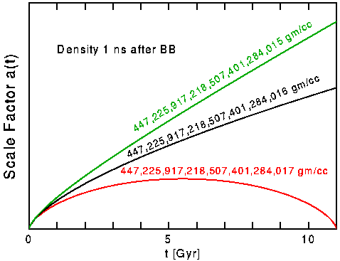
The figure above shows a(t) for three models with three different densities
at a time 1 nanosecond after the Big Bang. The black curve shows a
critical density case that matches the WMAP-based concordance model,
which has density = 447,225,917,218,507,401,284,016 gm/cc at
1 ns after the Big Bang.
Adding only 0.2 gm/cc to this 447 sextillion gm/cc causes the Big Crunch to
be right now! Taking away 0.2 gm/cc gives a model with a matter density
ΩM that is too
low for our observations. Thus the density 1 ns after the Big Bang
was set to an accuracy of better than 1 part in 2235 sextillion. Even
earlier it was set to an accuracy better than 1 part in 1059!
Since if the density is slightly high, the Universe will die in an early
Big Crunch, this is called the "oldness" problem in cosmology.
And since the critical density Universe has flat spatial geometry, it
is also called the "flatness" problem -- or the "flatness-oldness"
problem.
Whatever the mechanism for setting the density to equal the critical
density, it works extremely well, and it would be a remarkable coincidence
if Ωo were close to 1 but not exactly 1.
Note that the old version of this figure
was based on a model with higher current matter density, and also rounded
the true Δρ of 0.4 gm/cc to 1 based on rounding the logarithm.
Manipulating Space-Time Diagrams
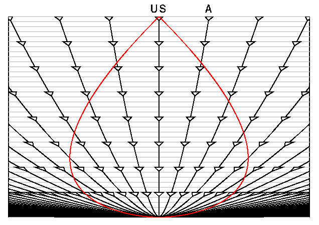
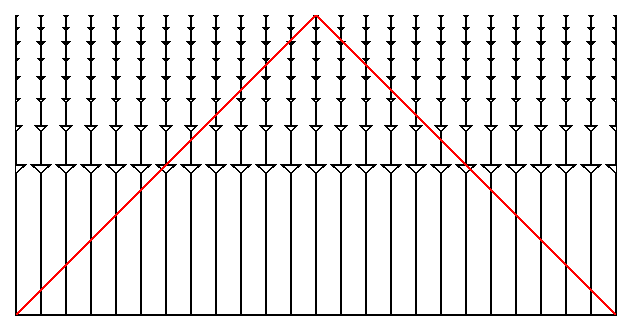
The critical density model is shown in the space-time diagram below.
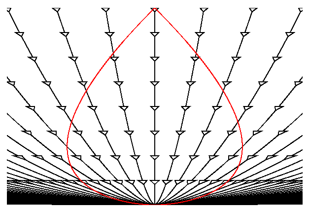
Note that the worldlines for galaxies are now curved due to the force of
gravity causing the expansion to decelerate. In fact, each worldline
is a constant factor times a(t) which is (t/to)2/3
for this Ωo = 1 model.
The red pearshaped object is our past lightcone.
While this diagram is drawn from our point-of-view, the Universe is
homogeneous so the diagram drawn from the point-of-view of any of the
galaxies on the diagram would be identical.
The diagram above shows the space-time diagram drawn on a deck of cards,
and the diagram below shows the deck pushed over to put it into A's
point-of-view.
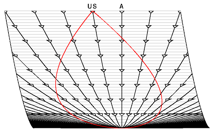
Note that this is not a Lorentz transformation, and that these
coordinates are not the special relativistic coordinates for which a
Lorentz transformation applies.
The Galilean transformation which
could be done by skewing cards in this way required that the edge of
the deck remain straight, and in any case the Lorentz transformation can
not be done on cards in this way because there is no absolute time.
But in cosmological models we do have cosmic time, which is the proper
time since the Big Bang measured by comoving observers, and it can be
used to set up a deck of cards.
The presence of gravity in this model
leads to a curved spacetime that can not be plotted on a flat space-time
diagram without distortion.
If every coordinate system is a distorted representation of the
Universe, we may as well use a convenient coordinate system and just
keep track of the distortion by following the lightcones.
Sometimes it is convenient to "divide out" the expansion of the
Universe, and the space-time diagram shows the result of dividing the
spatial coordinate by a(t). Now the worldlines of galaxies are all
vertical lines.
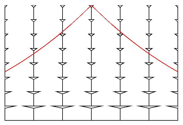
This division has expanded our past line cone so much that we have to
replot to show it all:
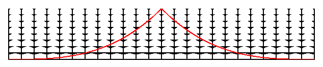
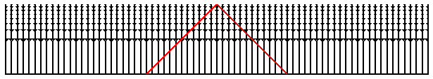
If we now "stretch" the time axis near the Big Bang we get the following
space-time diagram which has straight line past lightcones:
This kind of space-time diagram is called a "conformal" space-time
diagram, and while it is highly distorted it makes it easy to see where
the light goes. This transformation we have done is analogous to the
transformation from the side view of the Earth on the left below and the
Mercator chart on the right.
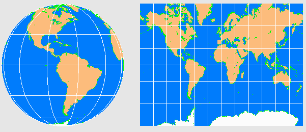
Note that a constant SouthEast course is a straight line on the Mercator
chart which is analogous to having straight line past lightcones on the
conformal space-time diagram.
Also remember that the Ωo = 1 spacetime is infinite in extent
so the conformal space-time diagram can go on far beyond our past
lightcone,
as shown above.
Other coordinates can be used as well. Plotting the spatial coordinate
as angle on polar graph paper makes the translation to a different
point-of-view easy. On the diagram below,
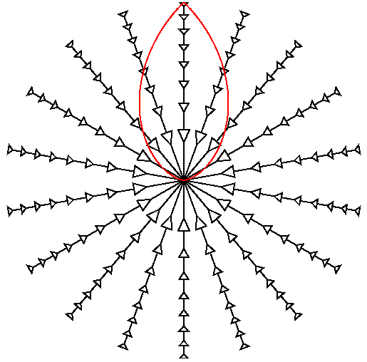
an Ωo = 2 model (which really is "round") is plotted this way with
a(t) used as the radial coordinate. The past lightcone of an observer
reachs halfway around the Universe in this model.
Horizon Problem
The conformal space-time diagram is a good tool use for describing the
meaning of CMB anisotropy observations. The Universe was opaque before
protons and electrons combined to form hydrogen atoms when the
temperature fell to about 3,000 K at a redshift of 1+z = 1090. After
this time the photons of the CMB have traveled freely through the
transparent Universe we see today. Thus the temperature of the CMB at a
given spot on the sky had to be determined by the time the hydrogen
atoms formed, usually called "recombination" even though it was the
first time so "combination" would be a better name.
Since the wavelengths in the CMB scale the same way that intergalaxy
distances do during the expansion of the Universe, we know that
a(t) had to be 0.0009 at recombination.
For the Ωo = 1 model this implies that
t/to = 0.00003 so for to about 14 Gyr the time is about
380,000 years after the Big Bang. This is such a small fraction of the
current age that the "stretching" of the time axis when making a
conformal space-time diagram is very useful to magnify this part of the
history of the Universe.
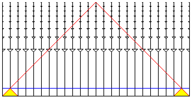
The conformal space-time diagram above has exaggerated this part even
further by taking the redshift of recombination to be 1+z = 144, which
occurs at the blue horizontal line. The yellow regions are the past
lightcones of the events which are on our past lightcone at
recombination. Any event that influences the temperature of the CMB
that we see on the left side of the sky must be within the left-hand
yellow region. Any event that affects the temperature of the CMB on the
right side of the sky must be within the right-hand yellow region.
These regions have no events in common, but the two temperatures are
equal to better than 1 part in 10,000. How is this possible?
This is known as the "horizon" problem in cosmology.
Next Section
Ned Wright's home page
FAQ |
Tutorial :
Part 1 |
Part 2 |
Part 3 |
Part 4 |
Age |
Distances |
Bibliography |
Relativity
© 1996-2009 Edward
L. Wright. Last modified 03 July 2009