Ned Wright's Cosmology Tutorial

Until a few hundred years ago, the Solar System and the Universe were equivalent in the minds of scientists, so the discovery that the Earth is not the center of the Solar System was an important step in the development of cosmology. Early in the 20th century Shapley established that the Solar System is far from the center of the Milky Way. So by the 1920's, the stage was set for the critical observational discoveries that led to the Big Bang model of the Universe.

Critical Observations

In 1929 Hubble [1, 2, 3] published a claim that the radial velocities of galaxies are proportional to their distance. The redshift of a galaxy is a measure of its radial velocity, and it can be measured using a spectrograph to determine the Doppler shift. The plot below shows Hubble's 1929 data:
Hubble's data

The slope of the fitted line is 464 km/sec/Mpc, and is now known as the Hubble constant, H_o. [Sometimes I will use "TeX" mode, so A_x means that x is a subscript, A_x, while A^x means that x is a superscript, A^x.] Since both kilometers and Megaparsecs (1 Mpc = 3.086E24 cm [the "E24" means multiply the 3.086 by 10 to the 24th power]) are units of distance, the simplified units of H_o are 1/time, and the conversion is given by

1/H_o = (978 Gyr)/(H_o in km/sec/Mpc)

Thus Hubble's value is equivalent to approximately 2 Gyr. Since this should be close to the age of the Universe, and we know (and it was known in 1929) that the age of the Earth is larger than 2 billion years, Hubble's value for H_o led to considerable skepticism about cosmological models, and motivated the Steady State model. However, later work found that Hubble had confused two different kinds of Cepheid variable stars used for calibrating distances, and also that what Hubble thought were bright stars in distant galaxies were actually H II regions. Correcting for these errors has led to a lowering of the value of the Hubble constant: there are now primarily two groups using Cepheids: the HST Distance Scale Key Project team (Freedman, Kennicutt, Mould etal) which gets 72+/-8 km/sec/Mpc, while the Sandage team, also using HST observations of Cepheids to calibrate Type Ia supernovae, gets 57+/-4 km/sec/Mpc. Other methods to determine the distance scale include the time delay in gravitational lenses and the Sunyaev-Zeldovich effect in distant clusters: both are independent of the Cepheid calibration and give values consistent with the average of the two HST groups: 65+/-8 km/sec/Mpc. These results are consistent with a combination of results from CMB anisotropy and the accelerating expansion of the Universe which give 71+/-3.5 km/sec/Mpc. With this value for H_o, the "age" 1/H_o is 14 Gyr while the actual age from the consistent model is 13.7+/-0.2 Gyr.

Hubble's data in 1929 is actually quite poor, since individual galaxies have peculiar velocities of several hundred km/sec, and Hubble's data only went out to 1200 km/sec. This has led some people to propose quadratic redshift-distance laws, but the data shown below on Type Ia SNe from Riess, Press and Kirshner (1996)

extend beyond 30,000 km/sec and provide a dramatic confirmation of the Hubble law,

v = dD/dt = H*D

The fitted line in this graph has a slope of 64 km/sec/Mpc. Since we measure the radial velocity using the Doppler shift, it is often called the redshift. The redshift z is defined such that:

1 + z = lambda(observed)/lambda(emitted)

where lambda is the wavelength of a line or feature in the spectrum of an object. We know from relativity that the redshift is given by

1 + z = sqrt((1+v/c)/(1-v/c))      so     v = cz + ...

The subscript "o" in H_o (pronounced "aitch naught") indicates the current value of a time variable quantity. Since the 1/H_o is approximately the age of the Universe, the value of H depends on time. Another quantity with a naught is t_o, the age of the Universe.

The linear distance-redshift law found by Hubble is compatible with a Copernican view of the Universe: our position is not a special one. First note that the recession velocity is symmetric: if A sees B receding, then B sees that A is receding, as shown in this diagram:

which is based on a sketch by Bob Kirshner. Then consider the following space-time diagram showing several nearby galaxies moving away from us from our point of view (galaxy A, the blue worldline) on the top and from galaxy B's (the green worldline) point of view on the bottom.
shift for linear law

The diagrams from the two different points of view are identical except for the names of the galaxies. The v(sq) = D² quadratic law, on the other hand, transforms into an anisotropic non-quadratic law when changing points of view, as shown below.
shift for square law

Thus if we saw a quadratic velocity vs. distance law, then an observer in a different galaxy would see a different law -- and one that would be different in different directions. Thus if we saw v(sq), then B would see much higher radial velocities in the "plus" direction than in the "minus" direction. This effect would allow one to locate the "center of Universe" by finding the one place where the redshift-distance law was the same in all directions. Since we actually see the same redshift-distance law in all directions, either the redshift-distance law is linear or else we are at the center which is anti-Copernican.

The Hubble law generates a homologous expansion which does not change the shapes of objects, while other possible velocity-distance relations lead to distortions during expansion.

The Hubble law defines a special frame of reference at any point in the Universe. An observer with a large motion with respect to the Hubble flow would measure blueshifts in front and large redshifts behind, instead of the same redshifts proportional to distance in all directions. Thus we can measure our motion relative to the Hubble flow, which is also our motion relative to the observable Universe. A comoving observer is at rest in this special frame of reference. Our Solar System is not quite comoving: we have a velocity of 370 km/sec relative to the observable Universe. The Local Group of galaxies, which includes the Milky Way, appears to be moving at 600 km/sec relative to the observable Universe.

Hubble also measured the number of galaxies in different directions and at different brightness in the sky. He found approximately the same number of faint galaxies in all directions, even though there is a large excess of bright galaxies in the Northern part of the sky. When a distribution is the same in all directions, it is isotropic. And when he looked for galaxies with fluxes brighter than F/4 he saw approximately 8 times more galaxies than he counted which were brighter than F. Since a flux 4 times smaller implies a doubled distance, and hence a detection volume that is 8 times larger, this indicated that the Universe is close to homogeneous (having uniform density) on large scales.

Homogeneous but not isotropic and vice-versa

The figure above shows a homogeneous but not isotropic pattern on the left and an isotropic but not homogeneous pattern on the right. If a figure is isotropic from more than 1 (2 if spherical) points, then it must also be homogeneous.

Of course the Universe is not really homogeneous and isotropic, because it contains dense regions like the Earth. But it can still be statistically homogeneous and isotropic, like this 24 kB simulated galaxy field, which is homogeneous and isotropic after smoothing out small scale details. Peacock and Dodds (1994, MNRAS, 267, 1020) have looked at the fractional density fluctuations in the nearby Universe as a function of the radius of a top-hat smoothing filter, and find:

delta(rho)/rho versus top-hat radius, H=65

Thus for 100 Mpc regions the Universe is smooth to within several percent. Redshift surveys of very large regions confirm this tendency toward smoothness on the largest scales, even though nearby galaxies show large inhomogeneities like the Virgo Cluster and the supergalactic plane.

The case for an isotropic and homogeneous Universe became much stronger after Penzias and Wilson announced the discovery of the Cosmic Microwave Background in 1965. They observed an excess flux at 7.5 cm wavelength equivalent to the radiation from a blackbody with a temperature of 3.7+/-1 degrees Kelvin. [The Kelvin temperature scale has degrees of the same size as the Celsius scale, but it is referenced at absolute zero, so the freezing point of water is 273.15 K.] A blackbody radiator is an object that absorbs any radiation that hits it, and has a constant temperature. Many groups have measured the intensity of the CMB at different wavelengths. Currently the best information on the spectrum of the CMB comes from the FIRAS instrument on the COBE satellite, and it is shown below:

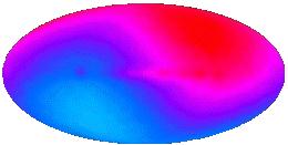
The x axis variable is the wavenumber or 1/[wavelength in cm]. The y axis variable is the power per unit area per unit frequency per unit solid angle in MegaJanskies per steradian. 1 Jansky is 10^-26 Watts per square meter per Hertz. The error bars have been multiplied by 400 so they can be seen, but the data points are consistent with the radiation from a blackbody with T_o = 2.725 K.

The temperature of the CMB is almost the same all over the sky. The figure below shows a map of the temperature on a scale where 0 K is black and 3 K is white.

Thus the microwave sky is extremely isotropic. These observations are combined into the Cosmological Principle:

The Universe is Homogeneous and Isotropic

Another piece of evidence in favor of the Big Bang is the abundance of the light elements, like hydrogen, deuterium (heavy hydrogen), helium and lithium. As the Universe expands, the photons of the CMB lose energy due to the redshift and the CMB becomes cooler. That means that the CMB temperature was higher in the past. When the Universe was only a few minutes old, the temperature was high enough to make the light elements by nuclear fusion. The theory of Big Bang Nucleosynthesis predicts that about 1/4 of the mass of the Universe should be helium, which is very close to what is observed. The abundance of deuterium is inversely related to the density of nucleons in the Universe, and the observed value of the deuterium abundance suggests that there is one nucleon for every 4 cubic meters of space in the the Universe.

Homogeneity and Isotropy

The Cosmological Principle:

The Universe is Homogeneous and Isotropic

To say the Universe is homogeneous means that any measurable property of the Universe is the same everywhere. This is only approximately true, but it appears to be an excellent approximation when one averages over large regions. Since the age of the Universe is one of the measurable quantities, the homogeneity of the Universe must be defined on a surface of constant proper time since the Big Bang. Time dilation causes the proper time measured by an observer to depend on the velocity of the observer, so we specify that the time variable t in the Hubble law is the proper time since the Big Bang for comoving observers.

Many Distances

With the correct interpretation of the variables, the Hubble law (v = HD) is true for all values of D, even very large ones which give v > c. But one must be careful in interpreting the distance and velocity. The distance in the Hubble law must be defined so that if A and B are two distant galaxies seen by us in the same direction, and A and B are not too far from each other, then the difference in distances from us, D(A)-D(B), is the distance A would measure to B. But this measurement must be made "now" -- so A must measure the distance to B at the same proper time since the Big Bang as we see now. Thus to determine D_now for a distant galaxy Z we would find a chain of galaxies ABC...XYZ along the path to Z, with each element of the chain close to its neighbors, and then have each galaxy in the chain measure the distance to the next galaxy at time t_o since the Big Bang. The distance to Z, D(us to Z), is the sum of all these subintervals:

D_now = D(us to Z) = D(us to A) + D(A to B) + ... D(X to Y) + D(Y to Z)

And the velocity in the Hubble law is just the change of D_now per unit time. It is close to cz for small redshifts but deviates for large ones. The space-time diagram below repeats the example from Part 1 showing how a change in point-of-view from observer A to observer B leaves the linear velocity vs. distance Hubble law unchanged:
linear v-vs-D
space-time with lightcones

linear v-vs-D
space-time with lightcones

but now showing the lightcones. Note how the lightcones must tip over along with the worldlines of the galaxies, showing that in these cosmological variables the speed of light is c with respect to local comoving observers.

The time and distance used in the Hubble law are not the same as the x and t used in special relativity, and this often leads to confusion. In particular, galaxies that are far enough away from us necessarily have velocities greater than the speed of light:

The light cones for distant galaxies in the diagram above are tipped over past the vertical, indicating v > c. The space-time diagram below shows a "zero" (really very low) density cosmological model plotted using the D_now and t of the Hubble law.
Omega=0 space-time

Worldlines of comoving observers are plotted and decorated with small, schematic lightcones. The red pear-shaped object is our past light cone. Notice that the red curve always has the same slope as the little light cones. In these variables, velocities greater than c are certainly possible, and since the open Universes are spatially infinite, they are actually required. But there is no contradiction with the special relativistic principle that objects do not travel faster than the speed of light, because if we plot exactly the same space-time in the special relativistic x and t coordinates we get:
Omega=0 model in SR coordinates

The grey hyperbolae show the surfaces of constant proper time since the Big Bang. When we flatten these out to make the previous space-time diagram, the worldlines of the galaxies get flatter and giving velocities v = dD_now/dt that are greater than c. But in special relativistic coordinates the velocities are less than c. We also see that our past light cone crosses the worldline of the most distant galaxies at a special relativistic distance x = c*t_o/2. But the Hubble law distance D_now, which is measured now, of these most distant galaxies is infinity (in this model). Furthermore, this galaxy with infinite Hubble law distance and hence infinite Hubble law velocity is visible to us, since in this model the observable Universe is the entire Universe. The relationships between the Hubble law distance and velocity (D_now & v) and the redshift z are given below:

v = H_oD_now
D_now = (c/H_o)ln(1+z)
1+z = exp(v/c)

Note that the redshift-velocity law is not the special relativistic Doppler shift law

1+z = sqrt[(1+v/c)/(1-v/c)]

which only applies to special relativistic coordinates, not to cosmological coordinates.

While the Hubble law distance is in principle measurable, the need for helpers all along the chain of galaxies out to a distant galaxy makes its use quite impractical. Other distances can be defined and measured more easily. One is the angular size distance, defined by

theta = size/D_A    so   D_A = size/theta

where "size" is the transverse extent of an object and "theta" is the angle (in radians) that it subtends on the sky. For the zero density model, the special relativistic x is equal to the angular size distance, x = D_A.

Another important distance indicator is the flux received from an object, and this defines the luminosity distance D_L through

Flux = Luminosity/(4*pi*D_L²)

A fourth distance is based on the light travel time: D_ltt = c*(t_o-t_em). People who say that the greatest distance we can see is c*t_o are using this distance. But D_ltt = c*(t_o-t_em) is not a very useful distance because it is very hard to determine t_em, the age of the Universe at the time of emission of the light we see. And finally, the redshift is a very important distance indicator, since astronomers can measure it easily, while the size or luminosity needed to compute D_A or D_L are always very hard to determine. The redshift is such a useful distance indicator that it is a shame that science journalists conspire to leave it out of stories: they must be taught the "5 w's but no z" rule in journalism school.

The predicted curve relating one distance indicator to another depends on the cosmological model. The plot of redshift vs distance for Type Ia supernovae shown earlier is really a plot of cz vs D_L, since fluxes were used to determine the distances of the supernovae. This data clearly rules out models that do not give a linear cz vs D_L relation for small cz. Extension of these observations to more distant supernovae have started to allow us to measure the curvature of the cz vs D_L relation, and provide more valuable information about the Universe.

The perfect fit of the CMB to a blackbody allows us to determine the D_A vs D_L relation. Since the CMB is produced at great distance but still looks like a blackbody, a distant blackbody must look like a blackbody (even though the temperature will change due to the redshift). The luminosity of blackbody is

L = 4*pi*R²*sigma*T_em⁴

where R is the radius, T_em is the temperature of the emitting blackbody, and sigma is the Stephan-Boltzmann constant. If seen at a redshift z, the observed temperature will be

T_obs = T_em/(1+z)

and the flux will be

F = theta²*sigma*T_obs⁴

where the angular radius is related to the physical radius by

theta = R/D_A

Combining these equations gives

D_L² = L/(4*pi*F)
    = (4*pi*R²*sigma*T_em⁴)/(4*pi*theta²*sigma*T_obs⁴)
    = D_A²*(1+z)⁴
      or
 D_L = D_A*(1+z)²

Models that do not predict this relationship between D_A and D_L, such as the chronometric model or the tired light model, are ruled out by the properties of the CMB.

Here is a Javascript calculator that takes H_o, Omega_M, the normalized cosmological constant lambda and the redshift z and then computes all of the these distances. Here are the technical formulae for these distances. The graphs below show these distances vs. redshift for three models: the critical density matter dominated Einstein - de Sitter model (EdS), the empty model, and the accelerating Lambda CDM model (LCDM) that is the current concensus model.

Note that all the distances are very similar for small distances, with D = cz/H_o, but the different types of distances deviate substantially at large redshifts. Also note that these deviations depend on what kind of Universe we live in. Precise measurements of deviations of D_L from cz/H_o are what tell us that the expansion of the Universe is accelerating.

Scale Factor a(t)

Because the velocity or dD_now/dt is strictly proportional to D_now, the distance between any pair of comoving objects grows by a factor (1+H*dt) during a time interval dt. This means we can write the distance to any comoving observer as

D_G(t) = a(t)*D_G(t_o)

where D_G(t_o) is the distance D_now to galaxy G now, while a(t) is universal scale factor that applies to all comoving objects. From its definition we see that a(t_o) = 1.

We can compute the dynamics of the Universe by considering an object with distance D(t) = a(t) D_o. This distance and the corresponding velocity dD/dt are measured with respect to us at the center of the coordinate system. The gravitational acceleration due to the spherical ball of matter with radius D(t) is g = -G*M/D(t)² where the mass is M = 4*pi*D(t)³*rho(t)/3. Rho(t) is the density of matter which depends only on the time since the Universe is homogeneous. The mass contained within D(t) is independent of the time since the interior matter has slower expansion velocity while the exterior matter has higher expansion velocity and thus stays outside. The gravitational effect of the external matter vanishes: the gravitational acceleration inside a spherical shell is zero, and all the matter in the Universe with distance from us greater than D(t) can be represented as union of spherical shells. With a constant mass interior to D(t) producing the acceleration of the edge, the problem reduces to the problem of a body moving radially in the gravitational field of a point mass. If the velocity is less than the escape velocity, the expansion will stop and recollapse. If the velocity equals the escape velocity we have the critical case. This gives

v = H*D = v(esc) = sqrt(2*G*M/D)
    H²*D² = 2*(4*pi/3)*rho*D²  or

rho(crit) = 3*H²/(8*pi*G)

For rho less than or equal to the critical density rho(crit), the Universe expands forever, while for rho greater than rho(crit), the Universe will eventually stop expanding and recollapse. The value of rho(crit) for H_o = 65 km/sec/Mpc is 8E-30 = 8*10^-30 gm/cc or 5 protons per cubic meter or 1.2E11 = 1.2*10¹¹ solar masses per cubic Megaparsec. The latter can be compared to the observed 1.75E8 = 1.75*10⁸ solar luminosities per Mpc³, requiring a mass-to-light ratio of 700 in solar units to close the Universe. If the density is anywhere close to critical most of the matter must be too dark to be observed. Current density estimates suggest that the matter density is between 0.2 to 1 times the critical density, and this does require that most of the matter in the Universe is dark.

Spatial Curvature

One consequence of general relativity is that the curvature of space depends on the ratio of rho to rho(crit). We call this ratio Omega = rho/rho(crit). For Omega less than 1, the Universe has negatively curved or hyperbolic geometry. For Omega = 1, the Universe has Euclidean or flat geometry. For Omega greater than 1, the Universe has positively curved or spherical geometry. We have already seen that the zero density case has hyperbolic geometry, since the cosmic time slices in the special relativistic coordinates were hyperboloids in this model.

The figure above shows the three curvature cases plotted along side of the corresponding a(t)'s. These a(t) curves assume that the cosmological constant is zero, which is not the current standard model. Omega > 1 still corresponds to a spherical shape, but could expand forever even though the density is greater than the critical density because of the repulsive gravitational effect of the cosmological constant.

The age of the Universe depends on Omega_o as well as H_o. For Omega=1, the critical density case, the scale factor is

a(t) = (t/t_o)^2/3

and the age of the Universe is

t_o = (2/3)/H_o

while in the zero density case, Omega=0, and

a(t) = t/t_o         with       t_o = 1/H_o

If Omega_o is greater than 1 the age of the Universe is even smaller than (2/3)/H_o.
a(t) for Omega=0,1,2

The figure above shows the scale factor vs time measured from the present for H_o = 65 km/sec/Mpc and for Omega_o = 0 (green), Omega_o = 1 (black), and Omega_o = 2(red). The age of the Universe is 15, 10 and 8.6 Gyr in these three models. The recollapse of the Omega_o = 2 model occurs when the Universe is 11 times older than it is now, and all observations indicate Omega_o < 2, so we have at least 80 billion more years before any Big Crunch.

The value of H_o*t_o is a dimensionless number that should be 1 if the Universe is almost empty and 2/3 if the Universe has the critical density. In 1994 Freedman et al. (Nature, 371, 757) found H_o = 80 +/- 17 and when combined with t_o = 14.6 +/- 1.7 Gyr, we find that H_o*t_o = 1.19 +/- 0.29. At face value this favored the empty Universe case, but a 2 standard deviation error in the downward direction would take us to the critical density case. Since both the age of globular clusters used above and the value of H_o depend on the distance scale in the same way, an underlying error in the distance scale could make a large change in H_o*t_o. In fact, recent data from the HIPPARCOS satellite suggest that the Cepheid distance scale must be increased by 10%, and also that the age of globular clusters must be reduced by 20%. If we take the latest HST value for H_o = 72 +/- 8 (Freedman et al. 2001, ApJ, 553, 47) and the latest globular cluster ages giving t_o = 13.5 +/- 0.7 Gyr, we find that H_o*t_o = 0.99 +/- 0.12 which is consistent with an empty Universe, but also consistent with the accelerating Universe that is the current standard model.

Flatness-Oldness Problem

However, if Omega_o is sufficiently greater than 1, the Universe will eventually stop expanding, and then Omega will become infinite. If Omega_o is less than 1, the Universe will expand forever and the density goes down faster than the critical density so Omega gets smaller and smaller. Thus Omega = 1 is an unstable stationary point unless the expansion of the universe is accelerating, and it is quite remarkable that Omega is anywhere close to 1 now.

The figure above shows a(t) for three models with three different densities at a time 1 nanosecond after the Big Bang. The black curve shows the critical density case with density = 447,225,917,218,507,401,284,016 gm/cc. Adding only 1 gm/cc to this 447 sextillion gm/cc causes the Big Crunch to be right now! Taking away 1 gm/cc gives a model with Omega that is too low for our observations. Thus the density 1 ns after the Big Bang was set to an accuracy of better than 1 part in 447 sextillion. Even earlier it was set to an accuracy better than 1 part in 10⁵⁹! Since if the density is slightly high, the Universe will die in an early Big Crunch, this is called the "oldness" problem in cosmology. And since the critical density Universe has flat spatial geometry, it is also called the "flatness" problem -- or the "flatness-oldness" problem. Whatever the mechanism for setting the density to equal the critical density, it works extremely well, and it would be a remarkable coincidence if Omega_o were close to 1 but not exactly 1.

Manipulating Space-Time Diagrams

The critical density model is shown in the space-time diagram below.

Note that the worldlines for galaxies are now curved due to the force of gravity causing the expansion to decelerate. In fact, each worldline is a constant factor times a(t) which is (t/t_o)^2/3 for this Omega_o = 1 model. The red pearshaped object is our past lightcone. While this diagram is drawn from our point-of-view, the Universe is homogeneous so the diagram drawn from the point-of-view of any of the galaxies on the diagram would be identical.
Omega=1 on cards

The diagram above shows the space-time diagram drawn on a deck of cards, and the diagram below shows the deck pushed over to put it into A's point-of-view.
Omega=1 on skewed cards

Note that this is not a Lorentz transformation, and that these coordinates are not the special relativistic coordinates for which a Lorentz transformation applies. The Galilean transformation which could be done by skewing cards in this way required that the edge of the deck remain straight, and in any case the Lorentz transformation can not be done on cards in this way because there is no absolute time. But in cosmological models we do have cosmic time, which is the proper time since the Big Bang measured by comoving observers, and it can be used to set up a deck of cards. The presence of gravity in this model leads to a curved spacetime that can not be plotted on a flat space-time diagram without distortion. If every coordinate system is a distorted representation of the Universe, we may as well use a convenient coordinate system and just keep track of the distortion by following the lightcones.

Sometimes it is convenient to "divide out" the expansion of the Universe, and the space-time diagram shows the result of dividing the spatial coordinate by a(t). Now the worldlines of galaxies are all vertical lines.

$Omega=1 t vs X_{cm} diagram$
This division has expanded our past line cone so much that we have to replot to show it all:
$Omega=1 t vs X_{cm} diagram wide-field$
If we now "stretch" the time axis near the Big Bang we get the following space-time diagram which has straight line past lightcones:
Omega=1 conformal diagram

This kind of space-time diagram is called a "conformal" space-time diagram, and while it is highly distorted it makes it easy to see where the light goes. This transformation we have done is analogous to the transformation from the side view of the Earth on the left below and the Mercator chart on the right.
Side view vs Mercator Earth

Note that a constant SouthEast course is a straight line on the Mercator chart which is analogous to having straight line past lightcones on the conformal space-time diagram.

Also remember that the Omega_o = 1 spacetime is infinite in extent so the conformal space-time diagram can go on far beyond our past lightcone,

as shown above.

Other coordinates can be used as well. Plotting the spatial coordinate as angle on polar graph paper makes the translation to a different point-of-view easy. On the diagram below,

an Omega_o = 2 model (which really is "round") is plotted this way with a(t) used as the radial coordinate. The past lightcone of an observer reachs halfway around the Universe in this model.

Horizon Problem

The conformal space-time diagram is a good tool use for describing the meaning of CMB anisotropy observations. The Universe was opaque before protons and electrons combined to form hydrogen atoms when the temperature fell to about 3,000 K at a redshift of 1+z = 1090. After this time the photons of the CMB have traveled freely through the transparent Universe we see today. Thus the temperature of the CMB at a given spot on the sky had to be determined by the time the hydrogen atoms formed, usually called "recombination" even though it was the first time so "combination" would be a better name. Since the wavelengths in the CMB scale the same way that intergalaxy distances do during the expansion of the Universe, we know that a(t) had to be 0.0009 at recombination. For the Omega_o = 1 model this implies that t/t_o = 0.00003 so for t_o about 14 Gyr the time is about 380,000 years after the Big Bang. This is such a small fraction of the current age that the "stretching" of the time axis when making a conformal space-time diagram is very useful to magnify this part of the history of the Universe.

Omega_o = 1 conformal space-time diagram

The conformal space-time diagram above has exaggerated this part even further by taking the redshift of recombination to be 1+z = 144, which occurs at the blue horizontal line. The yellow regions are the past lightcones of the events which are on our past lightcone at recombination. Any event that influences the temperature of the CMB that we see on the left side of the sky must be within the left-hand yellow region. Any event that affects the temperature of the CMB on the right side of the sky must be within the right-hand yellow region. These regions have no events in common, but the two temperatures are equal to better than 1 part in 10,000. How is this possible? This is known as the "horizon" problem in cosmology.

Inflation

The "inflationary scenario", developed by Starobinsky and by Guth, offers a solution to the flatness-oldness problem and the horizon problem. The inflationary scenario invokes a vacuum energy density. We normally think of the vacuum as empty and massless, and we can determine that the density of the vacuum is less than 1E-30 gm/cc now. But in quantum field theory, the vacuum is not empty, but rather filled with virtual particles:

The space-time diagram above shows virtual particle-antiparticle pairs forming out of nothing and then annihilating back into nothing. For particles of mass m, one expects about one virtual particle in each cubical volume with sides given by the Compton wavelength of the particle, h/mc, where h is Planck's constant. Thus the expected density of the vacuum is rho = m⁴*c³/h³ which is rather large. For the largest elementary particle mass usually considered, the Planck mass M defined by 2*pi*G*M² = h*c, this density is 2E91 gm/cc. Thus the vacuum energy density is at least 121 orders of magnitude smaller than the naive quantum estimate, so there must be a very effective suppression mechanism at work. If a small residual vacuum energy density exists now, it leads to a "cosmological constant" which is one proposed mechanism to relieve the tight squeeze between the Omega_o=1 model age of the Universe, t_o = (2/3)/H_o = 10 Gyr, and the apparent age of the oldest globular clusters, 16+/-4 Gyr. The vacuum energy density can do this because it produces a "repulsive gravity" that causes the expansion of the Universe to accelerate instead of decelerate, and this increases t_o for a given H_o.

The inflationary scenario proposes that the vacuum energy was very large during a brief period early in the history of the Universe. When the Universe is dominated by a vacuum energy density the scale factor grows exponentially, a(t) = exp(H(t_o-t)). The Hubble constant really is constant during this epoch so it doesn't need the "naught". If the inflationary epoch lasts long enough the exponential function gets very large. This makes a(t) very large, and thus makes the radius of curvature of the Universe very large. The diagram below shows our horizon superimposed on a very large radius sphere on top, or a smaller sphere on the bottom. Since we can only see as far as our horizon, for the inflationary case on top the large radius sphere looks almost flat to us.

This solves the flatness-oldness problem as long as the exponential growth during the inflationary epoch continues for at least 100 doublings. Inflation also solves the horizon problem, because the future lightcone of an event that happens before inflation is expanded to a huge region by the growth during inflation.
Inflationary space-time diagram

This space-time diagram shows the inflationary epoch tinted green, and the future lightcones of two events in red. The early event has a future lightcone that covers a huge area, that can easily encompass all of our horizon. Thus we can explain why the temperature of the microwave background is so uniform across the sky.

Details: Large-Scale Structure and Anisotropy

Of course the Universe is not really homogeneous, since it contains dense regions like galaxies and people. These dense regions should affect the temperature of the microwave background. Sachs and Wolfe (1967, ApJ, 147, 73) derived the effect of the gravitational potential perturbations on the CMB. The gravitational potential, phi = -GM/r, will be negative in dense lumps, and positive in less dense regions. Photons lose energy when they climb out of the gravitational potential wells of the lumps:

Sachs-Wolfe effect conformal space-time diagram

This conformal space-time diagram above shows lumps as gray vertical bars, the epoch before recombination as the hatched region, and the gravitational potential as the color-coded curve phi(x). Where our past lightcone intersects the surface of recombination, we see a temperature perturbed by dT/T = phi/(3*c²). Sachs and Wolfe predicted temperature fluctuations dT/T as large as 1 percent, but we know now that the Universe is far more homogeneous than Sachs and Wolfe thought. So observers worked for years to get enough sensitivity to see the temperature differences around the sky. The first anisotropy to be detected was the dipole anisotropy by Conklin in 1969:

The map above is from COBE and is much better than Conklin's 2 standard deviation detection. The red part of the sky is hotter by (v/c)*T_o, while the blue part of the sky is colder by (v/c)*T_o, where the inferred velocity is v = 370 km/sec. This is how we measure the velocity of the Solar System relative to the observable Universe. It was another 23 years before the anisotropy predicted by Sachs and Wolfe was detected by Smoot \etal in 1992. The amplitude was 1 part in 100,000 instead of 1 part in 100:

The map above shows cosmic anisotropy (and detector noise) after the dipole pattern and the radiation from the Milky Way have been subtracted out. The anisotropy in this map has an RMS value of 30 microK, and if it is converted into a gravitational potential using Sachs and Wolfe's result and that potential is then expressed as a height assuming a constant acceleration of gravity equal to the gravity on the Earth, we get a height of twice the distance from the Earth to the Sun. The "mountains and valleys" of the Universe are really quite large.

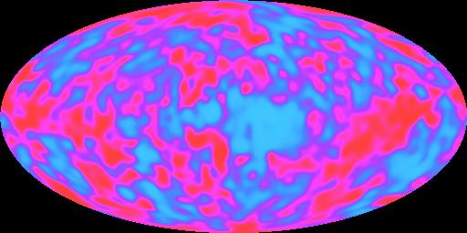
Inflation predicts a certain statistical pattern in the anisotropy. The quantum fluctuations normally affect very small regions of space, but the huge exponential expansion during the inflationary epoch makes these tiny regions observable.

Inflation generating equal power on all scales

The space-time diagram on the left above shows the future lightcones of quantum fluctuation events. The top of this diagram is really a volume which intersects our past lightcone making the sky. The future lightcones of events become circles on the sky. Events early in the inflationary epoch make large circles on the sky, as shown in the bottom map on the right. Later events make smaller circles as shown in the middle map, but there are more of them so the sky coverage is the same as before. Even later events make many small circles which again give the same sky coverage as seen on the top map.

An animated GIF file showing the spatial part of the above space-time diagram as a function of time is available here [1.2 MB].

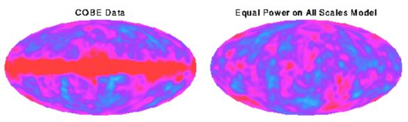
The pattern formed by adding all of the effects from events of all ages is known as "equal power on all scales", and it agrees with the COBE data.

Having found that the observed pattern of anisotropy is consistent with inflation, we can also ask whether the amplitude implies gravitational forces large enough to produce the observed clustering of galaxies.

phi(x) to clustering conformal space-time diagram

The conformal space-time diagram above shows the phi(x) at recombination determined by COBE's dT data, and the worldlines of galaxies which are perturbed by the gravitational forces produced by the gradient of the potential. Matter flows "downhill" away from peaks of the potential (red spots on the COBE map), producing voids in the current distribution of galaxies, while valleys in the potential (blue spots) are where the clusters of galaxies form.

COBE was not able to see spots as small as clusters or even superclusters of galaxies, but if we use "equal power on all scales" to extrapolate the COBE data to smaller scales, we find that the gravitational forces are large enough to produce the observed clustering, but only if these forces are not opposed by other forces. If the all the matter in the Universe is made out of the ordinary chemical elements, then there was a very effective opposing force before recombination, because the free electrons which are now bound into atoms were very effective at scattering the photons of the cosmic background. We can therefore conclude that most of the matter in the Universe is "dark matter" that does not emit, absorb or scatter light. Furthermore, observations of distant supernovae have shown that most of the energy density of the Universe is a vacuum energy density (a "dark energy") like Einstein's cosmological constant that causes an accelerating expansion of the Universe. These strange conclusions have been greatly strengthened by temperature anisotropy data at smaller angular scales which was be provided by the Wilkinson Microwave Anisotropy Probe (WMAP) in 2003.

Ned Wright's home page